Notes:
This project consists of two components which you can view/download from my Github repository:
The Octave/Matlab component contains two .m script files. They generate the data that the other project component relies on. I created the Octave/Matlab .m files using Octave, a free, open source alternative to Matlab. Though Octave is designed to be compatible with Matlab, it sometimes fails to be so.
The C++ component relies on special (SSE3) instructions that are not available on all machine architectures. The code should compile and run as expected on Intel or AMD CPUs from 2010 or newer. Running the code on older machines will result in errors, or worse, unexpected behavior.
I had been leafing through some detailed documentation on assembly language instructions (that’s my idea of a good time, I guess…) when I noticed that the floating point trigonometric instructions, fsin, fcos, fsincos, fptan, and fpatan all incur latencies that are considerably larger than do other instructions. This appears to be the case for every machine architecture described in the documentation. Why? And, by the way, how do computers calculate sin(x) and other such functions?
The above linked to stackoverflow question leads down a pretty deep rabbit hole; the topic is apparently a controversial and interesting one to more than just myself. To summarize some of the responses from the stackoverflow page, CPUs have hardware implementations of the CORDIC algorithm for such computations. This is what is used to evaluate the fsin, fcos, etc. assembly instructions–the ones that incur so much latency. And as someone else has uncovered, this algorithm has potential issues with accuracy, as well. But that’s only half the story. Compilers (mostly) won’t map your high level language sin(x) instruction to the fsin assembly instruction, but will instead map it to an elaborate software algorithm that evaluates the function with a truncated Taylor series, or Chebyshev polynomial.
This inspired me to try my own hand at a sin(x) approximation algorithm. I wondered if I could write an algorithm that was faster than the CPU or compiler software implementations at the expense of a reasonable degree of accuracy. Also, I opted to restrict the domain of my approximation to the interval, 

Calculations:
A continuous least squares polynomial approximation begins with a polynomial of degree n, with unknown coefficients,

the function it is to approximate, 


The error function is optimized by taking a partial derivative with respect to each coefficient and solving when equal to zero

This yields an equation for each coefficient,
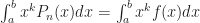
i.e.
For this project, the range in question is 

The vector on the right hand side has entries of the form

While these integrals can be solved with the product rule without any difficulty, they are tedious. I used Wolfram Alpha to get their closed form solutions. You can refer to my Octave sinApproxData.m source file to view them.
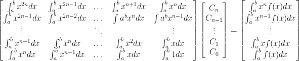
I solved systems for least square approximating polynomials of degrees two through eight. Here are my results:


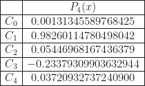


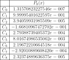
I noticed right away that the polynomials of odd degree are almost identical to their predecessors; their leading coefficients are nearly zero. This result surprised me. I at first speculated that this is to do with the Taylor series expansion of sin(x), since every other coefficient in the expansion is zero. But in its taylor series expansion, it’s the even coefficients that are zero, not the odd ones.
On the other hand, maybe its just that sin(x) on 
Here are some plots I made in octave of each approximating polynomial that has even degree, along with its squared difference from sin(x).

Since the polynomials of odd degree offer no improvement, their plots are omitted, however they can be found in the github repository associated with this project.

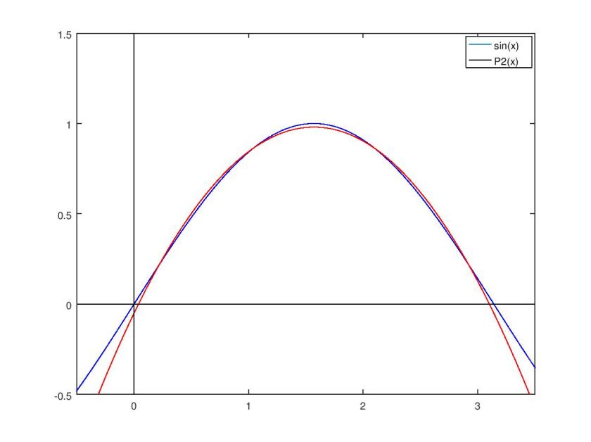
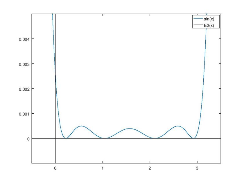

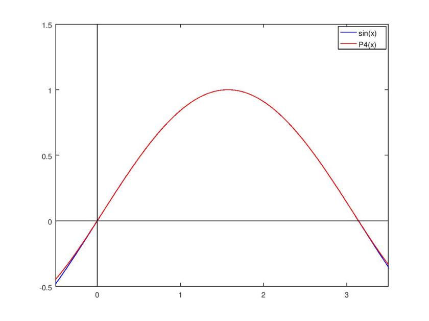


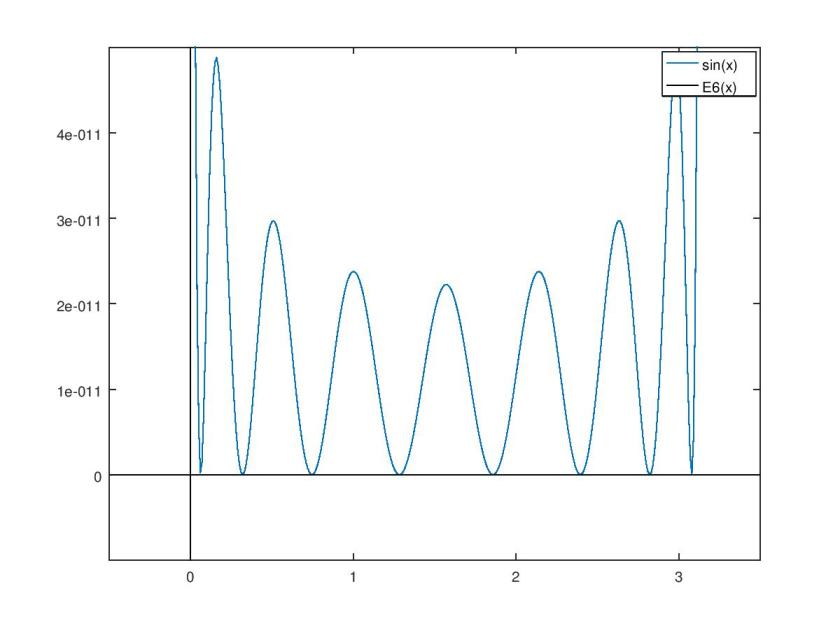


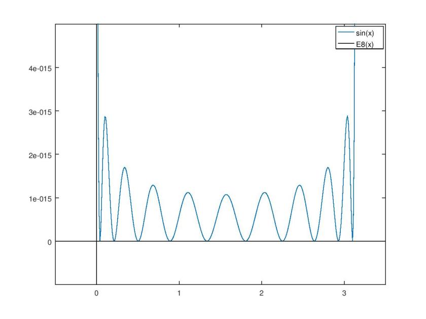
It’s clear that my chosen least squares method results in a lot of error near the boundaries of the approximation interval. While a least squares method minimizes the total error of the approximation, a Chebyshev polynomial approximation reduces error near the interval boundaries in exchange for a small increase in total error. In this regard, a Chebyshev polynomial approximation is probably a superior choice for practical applications.
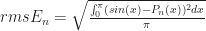
I calculated the root mean square error of each approximating polynomial to get an idea of how accurate I can expect it to be.

Implementation:
When it comes to evaluating polynomials, in general, Horner’s method is the most computationally efficient.
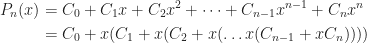
Straightforward evaluation of a polynomial of degree n requires n additions, n products, and n-1 exponentiations, whereas Horner’s method requires n additions, n products, and no exponentiation.
Breaking the process into partial steps yields the recurrence relation:

This translates easily into an algortihm. Here is my c++ implementation from this project. Note that in my implementation the coefficients are ordered in reverse.
double hornersMethod(double x, double* c, int length) {

	double y = 0;
	for (int i = 0; i < length; i++) {
		y = c[i] + x*y;
	}

	return y;
}
But this function is way too slow to compete with the built-in MSVC sin(x) function. First of all, it’s too general; coefficients and the number of them have to be passed to the function each time it is called. To remedy this issue, it’s necessary to make specialized functions for each particular polynomial that have the coefficients defined locally. I only did this for the polynomials of degree 4 and 8. I made another slight improvement with a technique called loop unrolling. Rather than iterating over a loop n times, the code within the loop are simply written n times. Normally this technique is redundant because a compiler will make this sort of optimization on it’s own. Here is my unrolled
double unrolledHornerSinP8(double x) {

	__declspec(align(16)) double c8[] = { 2.32374889636375e-005, -2.92010889608420e-004, 2.19672210664518e-004, 8.01674986535062e-003, 2.79388739405372e-004, -1.66810967472702e-001, 3.94059931985509e-005, 9.99995401622597e-001, 1.31570823227546e-007 };
	__declspec(align(16)) double y;

	y = c8[0];
	y = c8[1] + x*y;
	y = c8[2] + x*y;
	y = c8[3] + x*y;
	y = c8[4] + x*y;
	y = c8[5] + x*y;
	y = c8[6] + x*y;
	y = c8[7] + x*y;
	y = c8[8] + x*y;

	return y;
}
Having conducted some timings at this stage in development, I found that even this approach can’t compete. Then it dawned on me: factor–back to Octave!


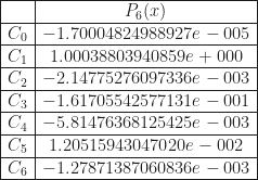
While
![\begin{aligned} (x-r_1)(x-r_2) &= x^2 - (r_1 + r_2)x + r_1 r_2 \\ &= x^2 - ([a+bi] + [a-bi])x + [a+bi][a-bi] \\ &= x^2 - 2ax + a^2+b^2 \end{aligned}](https://s0.wp.com/latex.php?latex=%5Cbegin%7Baligned%7D+%28x-r_1%29%28x-r_2%29+%26%3D+x%5E2+-+%28r_1+%2B+r_2%29x+%2B+r_1+r_2+%5C%5C+%26%3D+x%5E2+-+%28%5Ba%2Bbi%5D+%2B+%5Ba-bi%5D%29x+%2B+%5Ba%2Bbi%5D%5Ba-bi%5D+%5C%5C+%26%3D+x%5E2+-+2ax+%2B+a%5E2%2Bb%5E2+%5Cend%7Baligned%7D&bg=ffffff&fg=1a1a1a&s=0&c=20201002)
Here’s my factored
double factoredP8Sin(double x) {

	__declspec(align(16)) double r4[] = { 5.895452530035389, 3.141592785174156, -2.753860092985270, -0.000000131571428 };
	__declspec(align(16)) double q1[] = { -13.1185097003180, 48.6766343231151 };
	__declspec(align(16)) double q2[] = { 6.83532455770833, 17.3332241883087 };
	__declspec(align(16)) double r8Magnitude = 2.32374889636375e-005;

	return r8Magnitude*(x - r4[0])*(x - r4[1])*(x - r4[2])*(x - r4[3])*(x*x + q1[0] * x + q1[1])*(x*x + q2[0] * x + q2[1]);
}
While the public intrigue and controversy over the CPU trigonometric functions and their various compiler software alternatives that I stumbled upon initially got me thinking about this project, I decided to go ahead with it because I wanted an excuse to tinker around with SIMD (Single Instruction Multiple Data) assembly instructions. I had originally intended to write full on inline assembly routines, but I didn’t have the patience to figure out how to use some of the instructions necessary to do so (I found the shuffle instructions rather complex and tedious). Visual Studio provides an alternative means of accessing these instructions that allowed me to skirt around my lack of know how: intrinsics. As an afterthought, had I gone for full on inline assembly implementations of these algorithms, I probably would have gotten poor results in their timings; the MSVS compiler won’t optimize code within asm blocks, but it can optimize around intrinsics.
The SIMD instructions do as the acronym says; more than one variable can be loaded into a single SIMD register, a mathematical operation is performed with that register and another SIMD register, and the result is that operation performed on each individual variable within the register. This process is sometimes called vectorization. Since I was using 64-bit double precision variables in this project, there’s room for only two of them per SIMD register, but they could accommodate more than just two variables of lesser bit-width.
There are a ton of these SIMD instructions, but I wound up using just a few of them:
- _mm_add_pd(u, v)
- Add packed double precision values in registers u and v.
- _mm_mul_pd(u, v)
- Multiply packed double precision values in registers u and v.
- _mm_hadd_pd(u, v)
- Add packed doubles in register v together and place in lower half of result register, and add packed doubles in register u together and place in upper half of result register.
I wrote vectorized SIMD alternates of all my c++ functions. Most of these were boring, because they were just straightforward O(1) number crunching procedures. The general Horner’s method algorithm was interesting to write because it was a little more complex to begin with. I devised of splitting the polynomial in half, whereby the even terms of the polynomial are all evaluated in the lower half of a SIMD register, while the odd terms are evaluated in its upper half.
double hornersMethodSIMD(double x, double* c, unsigned int length) {

	__m128d u, v, w;

	u.m128d_f64[0] = x*x;
	u.m128d_f64[1] = x*x;						//u = | x^2 | x^2 |

	w.m128d_f64[0] = c[0];
	w.m128d_f64[1] = c[1];						//w = | c[1] | c[0] |

	for (int i = 2; i < (length - 1); i += 2) {
		v.m128d_f64[0] = c[i];
		v.m128d_f64[1] = c[i + 1];				//v = | c[i+1] | c[i] |
		w = _mm_mul_pd(u, w);					//w = | (x^2)*w[1] | (x^2)*w[0] |
		w = _mm_add_pd(v, w);					//w = | c[i+1] + x*w[1] | c[i] + x*w[0] |
	}

	if ((length % 2) == 0) {
		w.m128d_f64[0] *= x;					//w = | w[1] | x*w[0] |
	}
	else {
		u.m128d_f64[0] = x*x;
		u.m128d_f64[1] = x;						//u = | x | x^2 |
		w = _mm_mul_pd(u, w);					//w = | x*w[1] | (x^2)*w[0] |
		w.m128d_f64[0] += c[length - 1];		//w = | w[1] | c[n] + w[0] |
	}
	w = _mm_hadd_pd(w, w);						//w = | w[0]+w[1] | w[0]+w[1] |

	return w.m128d_f64[0];
}
Timings:
I first conducted timings on my computer with the compiler set to debug mode. This prevents the compiler from conducting optimization. Then I conducted the same timings again with the compiler set to release mode. This allows MSVS to optimize.


As for algorithm accuracy, I concede that my least square method is probabbly less desireable than what a Chebychev polynomial approximation could offer. Near the boundaries of the approximation, my approximations loose about a digit of accuracy. As for algorithm speed, the optimal code from this project came from both my efforts and those of the MSVS compiler working in tandem. When the compiler is allowed to optimize my c++ code, it actually does so with vectorized SIMD instructions. What it can’t do, however, is recognize the underlying task and design a vectorized algorithm to solve it. At least for now, that’s something only humans brains can do.
